
ABIGX: Explaining Why Industrial AI Detects a Fault
Published:
A model can detect an anomaly or classify a fault. But can it tell an engineer which variables actually drove that decision?
In our IEEE TPAMI 2026 paper, we introduce ABIGX (Adversarial fault reconstruction-Based Integrated Gradient eXplanation), a unified explanation framework for fault detection and fault classification. Its central idea is to reconstruct a meaningful fault-suppressing counterfactual and then attribute the model’s prediction relative to that reconstruction.
Paper: IEEE TPAMI, 48(9), 10906–10923 (2026) · Preprint · Code
Why explainable fault diagnosis needs a new framework
Industrial fault detection and classification (FDC) typically involves two questions:
- Detection: Is the process operating abnormally?
- Classification: If it is abnormal, which fault type is present?
A good diagnostic explanation must ask a third question: which input variables were responsible for the model’s fault prediction?
Classical tools such as contribution plots (CP) and reconstruction-based contributions (RBC) answer this question for traditional process-monitoring systems. However, their well-established formulations are closely tied to linear models such as principal component analysis (PCA), and many nonlinear extensions are specific to individual model architectures or restricted to detection. Meanwhile, general-purpose explainers such as Integrated Gradients (IG) depend on their baseline; an all-zero sensor reading may have no meaningful interpretation as a healthy process.
We wanted an approach that would preserve the physical diagnostic intuition of reconstruction, work with modern differentiable models, and explain both detection scores and classification decisions.
Key idea: reconstruct a fault before explaining it
ABIGX contains two stages:
Stage 1 — Adversarial Fault Reconstruction (AFR)
Traditional fault reconstruction changes a selected variable and searches for an adjustment that reduces a fault-detection index. We show that this has the same optimization objective as a sparse adversarial attack on a faulty sample when only that variable can be changed.
This observation motivates AFR: rather than searching one variable at a time, optimize a constrained input perturbation to suppress the abnormal signal. The reconstruction is guided by the learned FDC model and can account for interactions among variables.
For a fault detector, the objective is based on the squared prediction error (SPE) between the input and the model’s reconstruction. For a fault classifier, we introduce a representation-space classification SPE:
\[\mathrm{SPE}_{\mathrm{FC}}(x) = \left\|h(x)-\mathbb{E}_{x_n\sim X_{\mathrm{normal}}}[h(x_n)]\right\|_2^2,\]where (h(x)) is a learned representation (the penultimate layer by default). The goal is to move a faulty input toward the normal-data representation center, subject to a perturbation constraint. In the paper we explore optimization formulations and use projected gradient descent for general neural-network models.
Importantly, the AFR result is an approximate projection toward model-defined normality, not a guarantee of a physically realizable sample on the true data manifold.
Stage 2 — Integrated Gradient eXplanation (IGX)
The AFR-reconstructed sample becomes the adaptive baseline for IG. For an input (x), its AFR baseline (x’), and the FDC model quantity (F(x)), the contribution of variable (i) is:
\[\mathrm{ABIGX}_i=(x_i-x'_i)\int_0^1 \frac{\partial F(x'+\alpha(x-x'))}{\partial x_i}\,d\alpha.\]ABIGX thus explains the model by examining the transition from a model-informed, fault-suppressed reference back to the observed fault. Compared with a fixed zero baseline or an unrelated normal sample, this makes the attribution more specific to the fault instance.
What is theoretically new?
1. Classical CP and RBC are special cases
For PCA-based fault detection, we prove two exact identities under the corresponding reconstruction constructions:
- With the standard multivariable AFR reconstruction based on the residual projection, ABIGX is identical to CP.
- With one-variable AFR (ABIGX-OneVar), ABIGX is identical to RBC.
This establishes a theoretical bridge from classical industrial fault diagnosis to attribution for general differentiable FDC models. ABIGX is not simply an unexplained add-on to existing diagnostics: the classical methods appear naturally within the broader framework.
2. Fault-class smearing in fault classification
We identify and analyze fault-class smearing: a classifier must separate different fault types as well as distinguish faults from normal operation, and its class-discriminative weights can assign importance to variables belonging to other fault types.
As a result, gradient-based explanations may highlight irrelevant variables even when the classifier is trained optimally. We formally analyze this effect in a constructed linear classification setting. Under that setup, we prove that the fault-class smearing degree of ABIGX is lower than that of conventional IG.
The underlying insight is important beyond industrial monitoring: a feature that helps discriminate among classes is not necessarily the variable that produced the specific anomaly being explained.
Experiments: from industrial sensors to vision transformers
We evaluated ABIGX against classical contribution methods and modern XAI techniques with correctness metrics (alignment with fault-related variables or regions) and consistency metrics (whether adding/deleting important features changes the model prediction as expected).
| Application | Model family | What the explanation reveals |
|---|---|---|
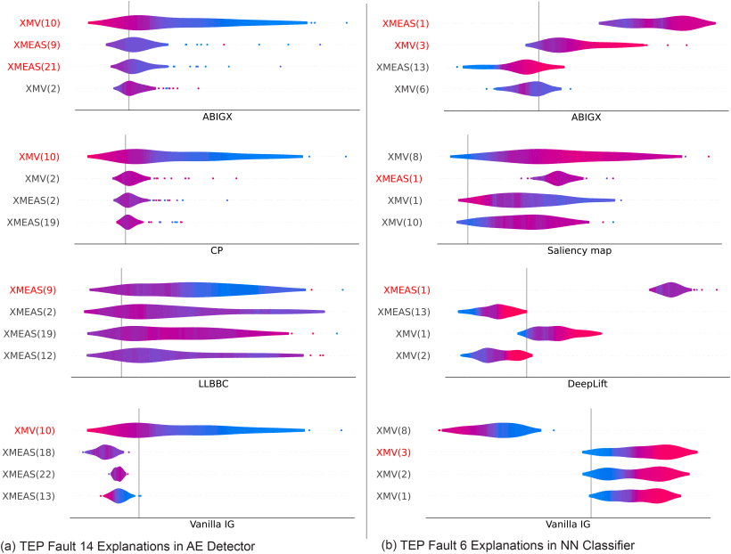
| Tennessee Eastman Process (TEP) | PCA, autoencoder, neural classifier | Sensor/actuator contributions for process faults; empirical agreement with CP/RBC in their linear settings |
| WM-811K semiconductor wafer maps | CNN | Image pixels that drive the classification of wafer failure patterns |
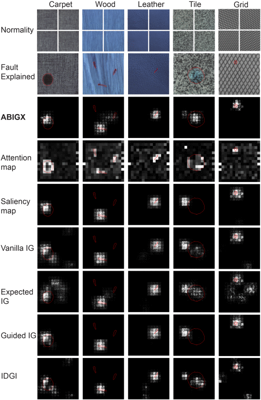
| MVTec-AD industrial images | WinCLIP with a differentiable ViT backbone | Localized visual regions behind anomaly detection decisions |
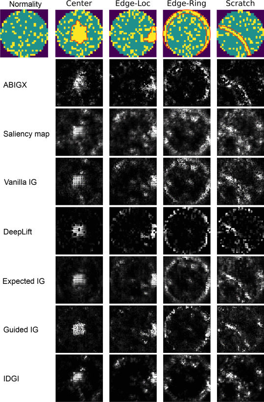
A concrete result: On the wafer-map CNN experiment, ABIGX achieved 0.839 correctness AUC and 0.859 consistency-ADD, versus 0.706 and 0.699 for vanilla IG (Table V of the paper). The AFR + Guided IG ablation is competitive and slightly exceeds ABIGX on some metrics, reinforcing that the counterfactual baseline itself is a major contributor to attribution quality.
The results on TEP likewise illustrate the benefits of fault-aware reconstruction. For example, in TEP Fault 6, ABIGX highlights XMEAS(1) and XMV(3), which are among the fault-related process variables, whereas several alternative explainers miss one of these signals. In visual inspection, attribution maps are more concentrated around relevant wafer-map and surface-defect regions.
What ABIGX does—and does not—claim
ABIGX provides feature attributions for the predictions of a trained FDC model. These can narrow down candidate fault sources and support engineering investigation; they are not certified causal root causes. Counterfactual reconstruction can also fail when the representation is poorly behaved or optimization does not reach a sufficiently normal-like reference. Iterative optimization and gradients add computational cost, particularly for large transformers, and access to differentiable model behavior is required.
These limits matter when moving from convincing attribution maps to trustworthy engineering decisions.
The bigger picture: IG² and ABIGX
My earlier work, IG²: Integrated Gradient on Iterative Gradient Path for Feature Attribution (TPAMI 2024), rethinks both the path and baseline of feature attribution using counterfactual gradients. ABIGX develops a complementary idea for industrial AI: derive the baseline from the fault-diagnosis task itself, then use IG to expose which variables support the decision.
Together, the two papers study a common principle: meaningful counterfactuals make feature attribution more informative.
Citation
Y. Zhuo, J. Qian, J. Zheng, X. Jiang, Z. Song, D. Chen, W. Yu, and Z. Ge, “ABIGX: A Unified Framework for Explainable Fault Detection and Classification,” IEEE Transactions on Pattern Analysis and Machine Intelligence, vol. 48, no. 9, pp. 10906–10923, 2026. DOI: 10.1109/TPAMI.2026.3689327.